Composite shapes
The basic usage of shapes was explained in the Finite size section of the tutorial. An overview of all the classes and function is available in the Shapes API reference. This section show how multiple of those shapes can be composed to quickly create intricate systems.
Download this page as a Jupyter notebook
Moving shapes
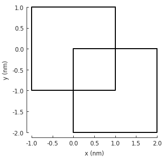
All shapes have a with_offset() method which simply translates the shape
by a vector:
shape = pb.rectangle(2, 2)
translated_shape = shape.with_offset([1, -1])
shape.plot()
translated_shape.plot()
This applies to any kind of shape, including user-defined freeform shapes:
def circle(radius):
    def contains(x, y, z):
        return np.sqrt(x**2 + y**2) < radius
    return pb.FreeformShape(contains, width=[2*radius, 2*radius])

shape = circle(1)
translated_shape = shape.with_offset([1, 0])
shape.plot()
translated_shape.plot()
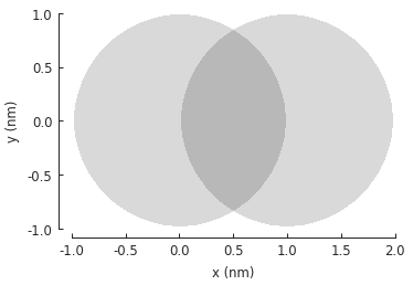
Note that Polygon and FreeformShape are presented differently in the plots.
For polygons, a line which connects all vertices is plotted. Freeform shapes are shown as a
lightly shaded silhouette which is filled in by calling the contains function and placing
dark pixels at positions where it returned True.
Using set operations
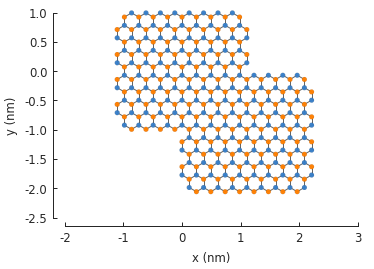
In the examples above we placed 2 shapes so that they overlap, but those were only plots. In order to create a composite shape, we can use logical and arithmetic operator. For example, addition:
s1 = pb.rectangle(2.3, 2.15)
s2 = s1.with_offset([1.12, -1.05])

composite_shape = s1 + s2
composite_shape.plot()
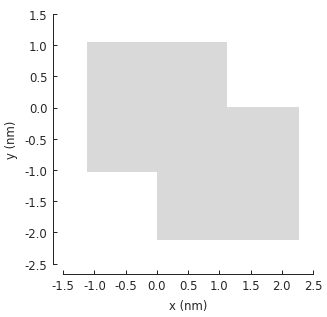
Note that even though we have combined two polygons, the composite shape is plotted in the style of a freeform shape. This is intentional to allow making completely generic shapes.
The + operator creates a union of the two shapes and the result can be used with a model:
from pybinding.repository import graphene

model = pb.Model(graphene.monolayer(), composite_shape)
model.plot()
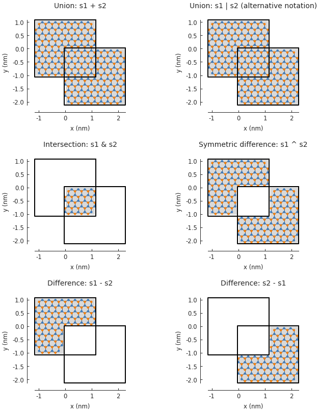
Shapes are composed in terms of set operations (e.g. unions, intersections) and the syntax mirrors
that of Python’s builtin set. The available operators and their results are shown in the code
and figure below. Note that the + and | operators perform the same function (union). Both
are available simply for convenience. Apart from -, all the operators are symmetric.
grid = plt.GridSpec(3, 2, hspace=0.4)
plt.figure(figsize=(6.7, 8))

titles_and_shapes = [
    ("Union: s1 + s2",                          s1 + s2),
    ("Union: s1 | s2 (alternative notation)",   s1 | s2),
    ("Intersection: s1 & s2",                   s1 & s2),
    ("Symmetric difference: s1 ^ s2",           s1 ^ s2),
    ("Difference: s1 - s2",                     s1 - s2),
    ("Difference: s2 - s1",                     s2 - s1)
]

for g, (title, shape) in zip(grid, titles_and_shapes):
    plt.subplot(g, title=title)
    s1.plot()
    s2.plot()
    model = pb.Model(graphene.monolayer(), shape)
    model.shape.plot()
    model.plot()
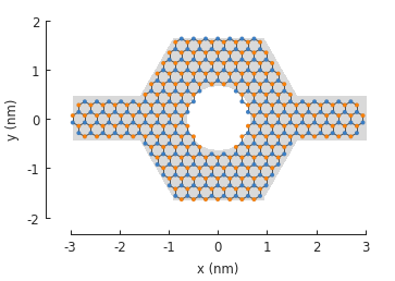
This isn’t limited to just two operands. Any number of shapes can be freely combined:
from math import pi

rectangle = pb.rectangle(x=6, y=1)
hexagon = pb.regular_polygon(num_sides=6, radius=1.92, angle=pi/6)
circle = pb.circle(radius=0.6)

model = pb.Model(
    graphene.monolayer(),
    (rectangle + hexagon) ^ circle
)
model.shape.plot()
model.plot()
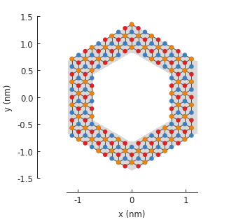
Additional examples
Circular rings are easy to create even with a FreeformShape, but composites make it
trivial to create rings as the difference of any two shapes:
outer = pb.regular_polygon(num_sides=6, radius=1.4)
inner = pb.regular_polygon(num_sides=6, radius=0.8)
model = pb.Model(graphene.bilayer(), outer - inner)
model.shape.plot()
model.plot()
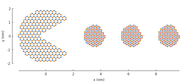
Of course, we can also go a bit wild:
plt.figure(figsize=(6.7, 2.6))

circle = pb.circle(radius=2)
triangle = pb.regular_polygon(num_sides=3, radius=2, angle=pi / 6).with_offset([1.4, 0])
pm = pb.Model(graphene.monolayer(), circle - triangle)
pm.plot()

dot = pb.circle(radius=0.8)
for x in [3.55, 6.25, 8.95]:
    pd = pb.Model(graphene.bilayer(), dot.with_offset([x, 0]))
    pd.plot()