Structure-mapped data
As shown in the previous section, many classes in pybinding use structure plots in a similar way.
One class stands out here: StructureMap can be used to map any arbitrary data onto the
spatial structure of a model. StructureMap objects are produced in two cases: as the
results of various computation functions (e.g. Solver.calc_spatial_ldos()) or returned
from Model.structure_map() which can map custom user data.
Download this page as a Jupyter notebook
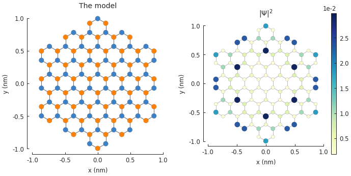
Draw only certain hoppings
Just as before, we can draw only the desired hoppings. Note that smap is a StructureMap
returned by Solver.calc_probability().
from pybinding.repository import graphene

plt.figure(figsize=(7, 3))

plt.subplot(121, title="The model")
model = pb.Model(graphene.monolayer(nearest_neighbors=3), graphene.hexagon_ac(1))
model.plot(hopping={'draw_only': ['t']})

plt.subplot(122, title="$|\Psi|^2$")
solver = pb.solver.arpack(model, k=10)
smap = solver.calc_probability(n=2)
smap.plot(hopping={'draw_only': ['t']})
pb.pltutils.colorbar()
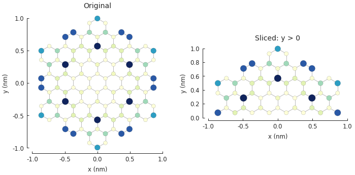
Slicing a structure
This follows a syntax similar to numpy fancy indexing where we can give a condition as the index.
plt.figure(figsize=(7, 3))

plt.subplot(121, title="Original")
smap.plot(hopping={'draw_only': ['t']})

plt.subplot(122, title="Sliced: y > 0")
upper = smap[smap.y > 0]
upper.plot(hopping={'draw_only': ['t']})
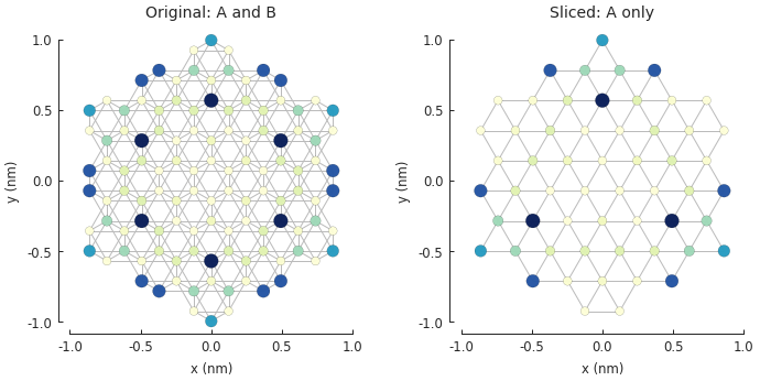
plt.figure(figsize=(7, 3))

plt.subplot(121, title="Original: A and B")
smap.plot(hopping={'draw_only': ['t', 't_nn']})

plt.subplot(122, title="Sliced: A only")
a_only = smap[smap.sublattices == 'A']
a_only.plot(hopping={'draw_only': ['t', 't_nn']})
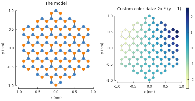
Mapping custom data
The method Model.structure_map() returns a StructureMap where any user-defined
data can be mapped to the spatial positions of the lattice sites. The data just needs to be
a 1D array with the same size as the total number of sites in the system.
plt.figure(figsize=(6.8, 3))

plt.subplot(121, title="The model")
model = pb.Model(graphene.monolayer(), graphene.hexagon_ac(1))
model.plot()

plt.subplot(122, title="Custom color data: 2x * (y + 1)")
custom_data = 2 * model.system.x * (model.system.y + 1)
smap = model.structure_map(custom_data)
smap.plot()
pb.pltutils.colorbar()
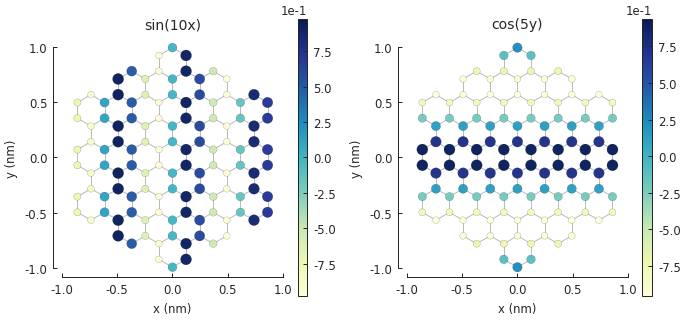
plt.figure(figsize=(6.8, 3))

plt.subplot(121, title="sin(10x)")
smap = model.structure_map(np.sin(10 * model.system.x))
smap.plot()
pb.pltutils.colorbar()

plt.subplot(122, title="cos(5y)")
smap = model.structure_map(np.cos(5 * model.system.y))
smap.plot()
pb.pltutils.colorbar()
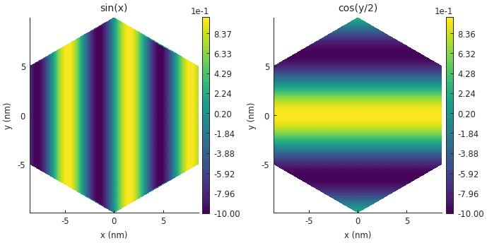
Contour plots for large systems
For larger systems, structure plots don’t make much sense because the details of the sites and hoppings would be too small to see. Contour plots look much better in this case.
plt.figure(figsize=(6.8, 3))
model = pb.Model(graphene.monolayer(), graphene.hexagon_ac(10))

plt.subplot(121, title="sin(x)")
smap = model.structure_map(np.sin(model.system.x))
smap.plot_contourf()
pb.pltutils.colorbar()

plt.subplot(122, title="cos(y/2)")
smap = model.structure_map(np.cos(0.5 * model.system.y))
smap.plot_contourf()
pb.pltutils.colorbar()
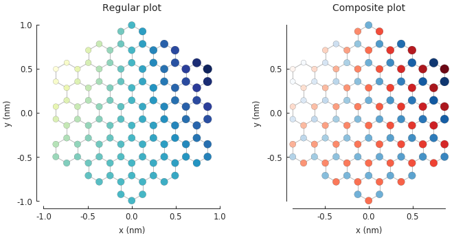
Composing multiple plots
Various plotting methods or even different invocations of the same method can be composed to create nice figures. For example, we may want to use different colormaps to distinguish between sublattices A and B when plotting some data on top of the structure of graphene. Below, the first pass plots only the hopping lines, the second pass draws the sites of sublattice A and the third draws sublattice B. The darkness of the color indicates the intensity of the mapped data, while blue/red distinguishes the sublattices.
model = pb.Model(graphene.monolayer(), graphene.hexagon_ac(1))
custom_data = 2 * model.system.x * (model.system.y + 1)
smap = model.structure_map(custom_data)

plt.figure(figsize=(6.8, 3))
plt.subplot(121, title="Regular plot")
smap.plot()

plt.subplot(122, title="Composite plot")
smap.plot(site_radius=0)  # only draw hopping lines, no sites
a_only = smap[smap.sublattices == "A"]
a_only.plot(cmap="Blues", hopping={'width': 0})  # A sites, no hoppings
b_only = smap[smap.sublattices == "B"]
b_only.plot(cmap="Reds", hopping={'width': 0})  # B sites, no hoppings