Multi-orbital models
In pybinding, if an onsite or hopping energy term is defined as a matrix (instead of a scalar), we refer to the resulting model as multi-orbital. The elements of the matrix term may correspond to different spins, electrons and holes, or any other degrees of freedom. These can have different physical meaning depending on the intend of the model. Because we’re talking in generic terms here, we’ll use orbital as a blanket term to refer to any degree of freedom, i.e. matrix element of an onsite or hopping term.
This section describes how these models can be defined and how the presence of multiple orbitals affects modifier functions and the results obtained from solvers. In general, it is as simple as replacing a scalar value with a matrix while all of the principals described in the Tutorial still apply.
Download this page as a Jupyter notebook
Onsite and hopping matrices
Starting from the very beginning, the orbital count of a site is determined by the shape of the onsite energy matrix. Let’s take a look at a few possibilities:
lat = pb.Lattice([1, 0], [0, 1])
lat.add_sublattices(
    ("A", [0.0, 0.0], 0.5),          # single-orbital: scalar
    ("B", [0.0, 0.2], [[1.5,  2j],   # two-orbital: 2x2 Hermitian matrix
                       [-2j, 1.5]]),
    ("C", [0.3, 0.1], np.zeros(2)),  # two-orbital: zero onsite term
    ("D", [0.1, 0.0], [[4, 0, 0],    # three-orbital: only diagonal
                       [0, 5, 0],
                       [0, 0, 6]]),
    ("E", [0.2, 0.2], [4, 5, 6])     # three-orbital: only diagonal, terse notation
)
The onsite term is required to be a square Hermitian matrix. If a 1D array is given instead of a matrix, it will be interpreted as the main diagonal of a square matrix (see sublattices D and E which have identical onsite term specified with different notations).
As seen above, sublattices don’t need to all have the same orbital count. The only thing to keep in mind is that the hopping matrix which connect a pair of sublattice sites must have the appropriate shape: the number of rows must match the orbital count of the source sublattice and the number of columns must match the destination sublattice.
lat.add_hoppings(
    ([0, 1], "A", "A", 1.2),          # scalar
    ([0, 1], "B", "B", [[1, 2],       # 2x2
                        [3, 4]]),
    ([0, 0], "B", "C", [[2j, 0],      # 2x2
                        [1j, 0]]),
    ([0, 0], "A", "D", [[1, 2, 3]]),  # 1x3
    ([0, 1], "D", "A", [[7],          # 3x1
                        [8],
                        [9]]),
    ([0, 0], "B", "D", [[1j, 0,  0],  # 2x3
                        [2,  0, 3j]])
)
If a matrix of the wrong shape is given, an informative error is raised:
>>> lat.add_one_hopping([0, 0], "A", "B", 0.6)
RuntimeError: Hopping size mismatch: from 'A' (1) to 'B' (2) with matrix (1, 1)
>>> lat.add_one_hopping([0, 1], "D", "D", [[1, 2, 3],
...                                        [4, 5, 6]])
RuntimeError: Hopping size mismatch: from 'D' (3) to 'D' (3) with matrix (2, 3)
After the Lattice is complete, a Model can be built as usual:
>>> model = pb.Model(lat, pb.primitive(2, 2))
>>> model.system.num_sites
20  # <-- 5 sites per unit cell and 2x2 cells: 5*2*2 == 20
>>> model.hamiltonian.shape
(44, 44)  # <-- 11 (1+2+2+3+3) orbitals per unit cell and 2x2 cells: 11*2*2 = 44
Sites refer to physical locations so their total count corresponds to the number of sublattices
(A to E) multiplied by the number of times the unit cell is repeated. The Hamiltonian matrix is
larger than num_sites due to the extra orbitals.
Effect on modifier functions
The @onsite_energy_modifier and
@hopping_energy_modifier functions work equally well for
single- and multi-orbital models. In case of the latter, the energy argument of the modifiers
will have a shape matching the onsite/hopping matrix term.
@pb.onsite_energy_modifier
def potential(energy, x):
    """Linear onsite potential as a function of x for a 2-orbital model"""
    return energy + np.eye(2) * x
Note the np.eye(2) in the code above. The number 2 matches the 2-orbital
structure of a specific model. Without this, energy + x would also add the value to the
off-diagonal elements of the onsite matrix which is not desirable in this case.
The modifier defined above will only work for 2-orbital models. In general, we might want to
create modifiers which work with any n-orbital model or with a mixed number of orbitals. For this
we can use the sub_id modifier argument and its .eye attribute which supplies the correct
matrix shape for any sublattice:
@pb.onsite_energy_modifier
def potential(energy, x, sub_id):
    """Same as above, but works for any n-orbital model"""
    return energy + sub_id.eye * x
Even more generally, if we wish to apply completely different functions to the various sublattices,
the sub_id argument can be used to create different branches in the modifier:
@pb.onsite_energy_modifier
def potential(energy, x, sub_id):
    """Applies different functions to different sublattices"""
    if sub_id == "A":
        return energy + x  # we know sublattice A is single-orbital
    elif sub_id == "D":
        energy[x > 0] += sub_id.eye * x  # the notation can be mixed with numpy indexing
        return energy                    # apply only to sites where x > 0
    elif sub_id == "B":
        sigma_y = np.array([[0, -1j],
                            [1j,  0]])
        return energy + sigma_y * 1.3 - np.eye(2) * 0.6  # add multiple 2x2 matrices
    else:
        return energy  # leave the other sublattices unchanged
This branching behavior is only supported by the sub_id and hop_id arguments. Do not try
to create branches like this using any of the other modifier arguments:
"""Creating a position-dependent potential"""
# This is an error with anything except sub_id or hop_id
if x > 0:
    return energy + 1
else:
    return energy - 1
# Use this notation instead
energy[x >  0] += 1
energy[x <= 0] -= 1
On the other hand, sub_id and hop_id can be used with either of these variants with just a
single caveat:
"""Sublattice-dependent potential"""
# This always works with sub_id and hop_id
if sub_id == "A":
    return energy + 1
else:
    return energy - 1
# This only works when all sublattices have the same number of orbitals,
# but it will raise an error for mixed orbital counts.
energy[sub_id == "A"] += 1
energy[sub_id == "B"] -= 1
Local properties and plotting
When examining the local properties of a multi-orbital model, it is important to make the distinction between system indices which correspond to sites (unique positions) and Hamiltonian indices which correspond to the onsite or hopping terms in the Hamiltonian.
As shown in one of the previous examples, the number of sites in a system does not have to be
equal to the size of the Hamiltonian matrix (hamiltonian.shape[0] >= num_sites). This affects
how the system and Hamiltonian are indexed. System indices are always scalars and point to a single
site position. For single-orbital models there is a 1:1 correspondence between system and
Hamiltonian indices. However, for multi-orbital models the Hamiltonian indices are 1D arrays with
a size corresponding to the number of orbitals on the target site.
>>> model = pb.Model(lat, pb.primitive(2, 2))
>>> sys_idx = model.system.find_nearest(position=[0, 0], sublattice="D")
>>> sys_idx  # <-- Points to a site on sublattice D which is closest to the target position.
15           #     It's always a scalar.
>>> model.system.x[sys_idx]
0.1  # <-- Not exactly 0 as requested, but the closest site to it.
>>> model.system.y[sys_idx]
0.0
>>> ham_idx = model.system.to_hamiltonian_indices(sys_idx)
>>> ham_idx   # <-- Array of integers which can be used to index the Hamiltonian matrix.
[29, 30, 31]  #     Size 3 because the selected site is on the 3-orbital sublattice D.
>>> ham = model.hamiltonian.todense()
>>> ham[np.ix_(ham_idx, ham_idx)]  # Returns the onsite hopping term of sublattice D.
[[4, 0, 0],
 [0, 5, 0],
 [0, 0, 6]]
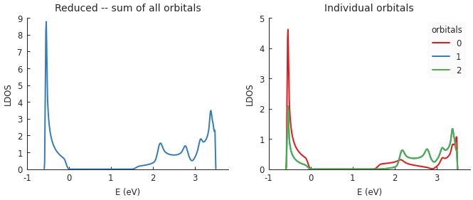
Functions which compute various local properties take into account the presence of multiple orbitals on a single site. For example, when calculating the local density of states, one of the input parameters is the target site position. By default, the resulting LDOS is calculated as the sum of all orbitals but this is optional as shown in the following example:
"""Calculate the LDOS in the center of a MoS2 quantum dot"""
from pybinding.repository import group6_tmd

model = pb.Model(group6_tmd.monolayer_3band("MoS2"),
                 pb.regular_polygon(6, 20))

kpm = pb.kpm(model)
energy = np.linspace(-1, 3.8, 500)
broadening = 0.05
position = [0, 0]

plt.figure(figsize=(6.7, 2.3))

plt.subplot(121, title="Reduced -- sum of all orbitals")
ldos = kpm.calc_ldos(energy, broadening, position)
ldos.plot(color="C1")

plt.subplot(122, title="Individual orbitals")
ldos = kpm.calc_ldos(energy, broadening, position, reduce=False)
ldos.plot()