3. Band structure
In order to calculate the band structure of a crystal lattice, this section introduces
the concepts of a Model and a Solver.
Download this page as a Jupyter notebook
3.1. Model
A Model contains the full tight-binding description of the physical system that we wish
to solve. We’ll start by assigning a lattice to the model, and we’ll use a pre-made one from the
material repository.
from pybinding.repository import graphene

model = pb.Model(graphene.monolayer())
model.plot()
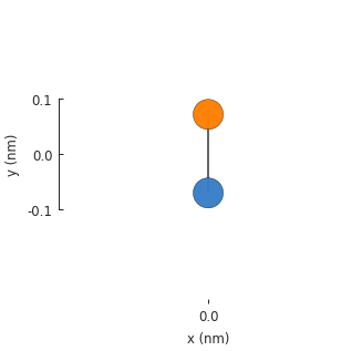
The result is not very exciting: just a single graphene unit cell with 2 atoms and a single
hopping between them. The model does not assume translational symmetry or any other physical
property. Given a lattice, it will just create a single unit cell. The model has a System
attribute which keeps track of structural properties like the positions of lattice sites and the
way they are connected, as seen in the figure above. The raw data can be accessed directly:
>>> model.system.x
[0, 0]
>>> model.system.y
[-0.071  0.071]
>>> model.system.sublattices
[0 1]
Each attribute is a 1D array where the number of elements is equal to the total number of lattice
sites in the system. The model also has a hamiltonian attribute:
>>> model.hamiltonian
(0, 1)   -2.8
(1, 0)   -2.8
It’s a sparse matrix (see scipy.sparse.csr_matrix) which corresponds to the tight-binding
Hamiltonian of our model. The output above shows the default sparse representation of the data
where each line corresponds to (row, col) value. Alternatively, we can see the dense matrix
output:
>>> model.hamiltonian.todense()
[[ 0.0 -2.8]
 [-2.8  0.0]]
Next, we include translational_symmetry() to create an infinite graphene sheet.
model = pb.Model(
    graphene.monolayer(),
    pb.translational_symmetry()
)
model.plot()
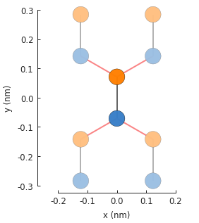
The red lines indicate hoppings on periodic boundaries. The lighter colored circles represent the translations of the unit cell. The number of translations is infinite, but the plot only presents the first one in each lattice vector direction.
3.2. Solver
A Solver can exactly calculate the eigenvalues and eigenvectors of a Hamiltonian matrix.
We’ll take a look at various Eigenvalue solvers and their capabilities in a later section, but right
now we’ll just grab the lapack() solver which is the simplest and most appropriate for
small systems.
>>> model = pb.Model(graphene.monolayer())
>>> solver = pb.solver.lapack(model)
>>> solver.eigenvalues
[-2.8 2.8]
>>> solver.eigenvectors
[[-0.707 -0.707]
 [-0.707  0.707]]
Beyond just the eigenvalues and eigenvectors properties,
Solver has a convenient calc_bands() method which can be used to
calculate the band structure of our model.
from math import sqrt, pi

model = pb.Model(graphene.monolayer(), pb.translational_symmetry())
solver = pb.solver.lapack(model)

a_cc = graphene.a_cc
Gamma = [0, 0]
K1 = [-4*pi / (3*sqrt(3)*a_cc), 0]
M = [0, 2*pi / (3*a_cc)]
K2 = [2*pi / (3*sqrt(3)*a_cc), 2*pi / (3*a_cc)]

bands = solver.calc_bands(K1, Gamma, M, K2)
bands.plot(point_labels=['K', r'$\Gamma$', 'M', 'K'])
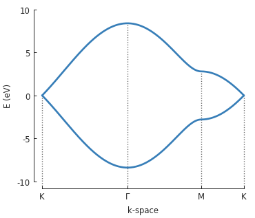
The points \(\Gamma, K\) and \(M\) are used to draw a path in the reciprocal space of
graphene’s Brillouin zone and Solver.calc_bands() calculates the band energy along
that path. The return value of the method is a Bands result object.
All result objects have built-in plotting methods. Aside from the basic plot() seen
above, Bands also has plot_kpath() which presents the path in reciprocal
space. Plots can easily be composed, so to see the path in the context of the Brillouin zone, we
can simply plot both:
model.lattice.plot_brillouin_zone(decorate=False)
bands.plot_kpath(point_labels=['K', r'$\Gamma$', 'M', 'K'])
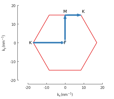
The extra argument for Lattice.plot_brillouin_zone() turns off the reciprocal lattice
vectors and vertex coordinate labels (as seen in the previous section).
Note
The band structure along a path in k-space can also be calculated manually by saving an
array of Solver.eigenvalues at different k-points. This process is shown on the
Eigensolver page.
3.3. Switching lattices
We can easily switch to a different material, just by passing a different lattice to the model.
For this example, we’ll use our pre-made graphene.bilayer()
from the Material Repository. But you can create any lattice as described in the previous
section: Lattice.
model = pb.Model(graphene.bilayer())
model.plot()
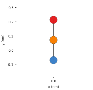
Without translational_symmetry(), the model is just a single unit cell with 4 atoms. Our
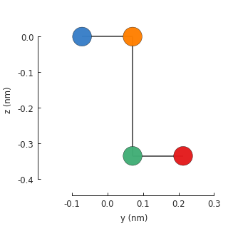
bilayer lattice uses AB-stacking where a pair of atoms are positioned one on top of the another.
By default, the Model.plot() method shows the xy-plane, so one of the bottom atoms isn’t
visible. We can pass an additional plot argument to see the yz-plane:
model = pb.Model(graphene.bilayer())
model.plot(axes='yz')
To compute the band structure, we’ll need to include translational_symmetry().
model = pb.Model(graphene.bilayer(), pb.translational_symmetry())
model.plot()
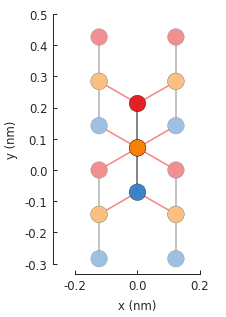
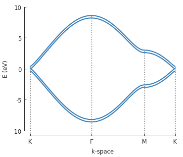
As before, the red hoppings indicate periodic boundaries and the lighter colored circles represent the first of an infinite number of translation units. We’ll compute the band structure for the same \(\Gamma\), \(K\) and \(M\) points as monolayer graphene:
solver = pb.solver.lapack(model)
bands = solver.calc_bands(K1, Gamma, M, K2)
bands.plot(point_labels=['K', r'$\Gamma$', 'M', 'K'])
3.4. Further reading
Check out the examples section for more band structure calculations with various other lattices. Eigenvalue solvers will be covered in more detail at a later point in the tutorial, but this is enough information to get started. The next few sections are going to be dedicated to model building.
3.5. Example
"""Calculate and plot the band structure of monolayer graphene"""
import pybinding as pb
import matplotlib.pyplot as plt
from math import sqrt, pi
from pybinding.repository import graphene

pb.pltutils.use_style()


model = pb.Model(
    graphene.monolayer(),  # predefined lattice from the material repository
    pb.translational_symmetry()    # creates an infinite sheet of graphene
)
solver = pb.solver.lapack(model)  # eigensolver from the LAPACK library

# significant points in graphene's Brillouin zone
a_cc = graphene.a_cc  # carbon-carbon distance
Gamma = [0, 0]
K1 = [-4*pi / (3*sqrt(3)*a_cc), 0]
M = [0, 2*pi / (3*a_cc)]
K2 = [2*pi / (3*sqrt(3)*a_cc), 2*pi / (3*a_cc)]

# plot the bands through the desired points
bands = solver.calc_bands(K1, Gamma, M, K2)
bands.plot(point_labels=['K', r'$\Gamma$', 'M', 'K'])
plt.show()
