11. Scattering model
This section introduces the ability to attach semi-infinite leads to a finite-sized central region, thereby creating a scattering model.
Download this page as a Jupyter notebook
11.1. Attaching leads
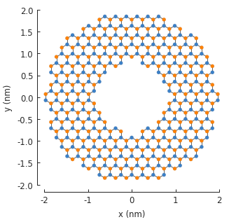
To start with, we need a finite-sized system to serve as the central scattering region. We’ll just make a simple ring. Refer to the Finite size section for more details.
from pybinding.repository import graphene

def ring(inner_radius, outer_radius):
    """A simple ring shape"""
    def contains(x, y, z):
        r = np.sqrt(x**2 + y**2)
        return np.logical_and(inner_radius < r, r < outer_radius)
    return pb.FreeformShape(contains, width=[2*outer_radius, 2*outer_radius])

model = pb.Model(graphene.monolayer(), ring(0.8, 2))
model.plot()
To attach a lead to this system, we call the Model.attach_lead() method:
model.attach_lead(direction=-1, contact=pb.line([-2, -1], [-2, 1]))

plt.figure(figsize=(6, 3))  # make the figure wider
model.plot()
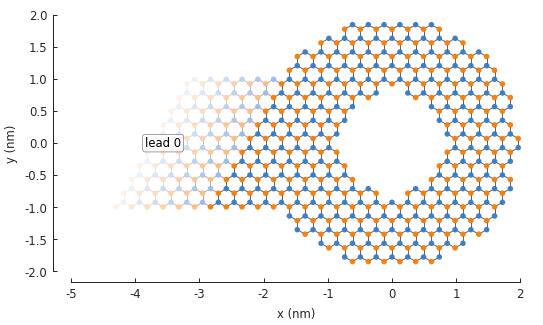
The lead is semi-infinite, but to be practical for the figure, only a few repetitions of the lead’s
unit cell are drawn. They fade out gradually along the direction where the lead goes to infinity.
The periodic hoppings between the unit cells are shown in red. The label indicates that this lead
has the index 0. It’s attributes can be accessed using this index and the Model.leads
list. The lead was created using two parameters: direction and the contact shape. To illustrate
the meaning of these parameters, we’ll draw them using the Lead.plot_contact() method:
plt.figure(figsize=(6, 3))  # make the figure wider
model.plot()
model.leads[0].plot_contact()  # red shaded area and arrow
model.lattice.plot_vectors(position=[-2.5, 1.5], scale=3)
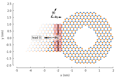
The direction of a lead is specified in terms of lattice vectors. In this case direction=-1
indicates that it should be opposite the \(a_1\) lattice vector, as shown in the figure with
the arrow labeled \(-a_1\). For 2D systems, the allowed directions are \(\pm1, \pm2\).
The position of the lead is chosen by specifying a contact shape. The intersection of a
semi-infinite lead and a 2D system is a 1D line, which is why we specified
contact=pb.line([-2, -1], [-2, 1]), where the two parameters given to line() are point
positions. The line is drawn in the figure above in the middle of the red shaded area (the red
area itself does not have any physical meaning, it’s just there to draw attention to the line).
Note
For a 3D system, the lead contact area would be 2D shape, which could be specified by
a Polygon or a FreeformShape.
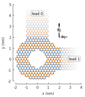
We can now proceed to attach a few more leads:
model.attach_lead(direction=+2, contact=pb.line([-1,  1.8], [1,  1.8]))
model.attach_lead(direction=+1, contact=pb.line([ 2, -1  ], [2,  1  ]))
model.attach_lead(direction=-2, contact=pb.line([-1, -1.8], [1, -1.8]))

plt.figure(figsize=(6.9, 6))
model.plot()
model.leads[1].plot_contact()
model.leads[2].plot_contact()
model.lattice.plot_vectors(position=[-2, 2], scale=3)
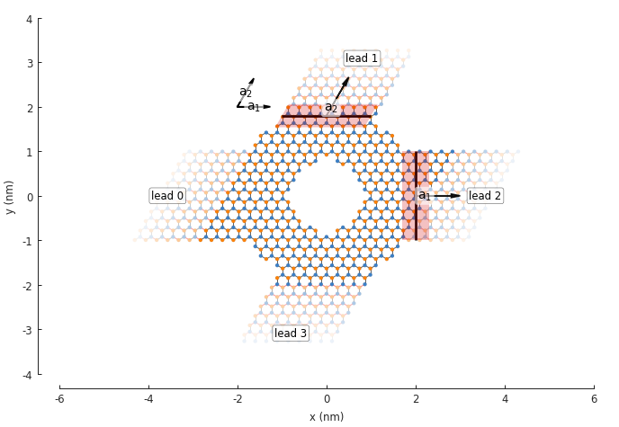
Notice that leads 1 and 3 are not perpendicular to leads 0 and 2. This is due to the angle of
the primitive lattice vectors \(a_1\) and \(a_2\), as shown in the same figure. All of
the leads also have zigzag edges because of this primitive vector arrangement. If we substitute
the regular graphene lattice with graphene.monolayer_4atom(),
the primitive vectors will be perpendicular and we’ll get different leads in the \(\pm2\)
directions:
model = pb.Model(graphene.monolayer_4atom(), ring(0.8, 2))
model.attach_lead(direction=+2, contact=pb.line([-1,  1.8], [1, 1.8]))
model.attach_lead(direction=+1, contact=pb.line([ 2, -1  ], [2, 1  ]))
model.plot()
model.lattice.plot_vectors(position=[2, 2], scale=3)
11.2. Lead attributes
The attached leads can be accessed using the Model.leads list. Each entry is a
Lead object with a few useful attributes. The unit cell of a lead is described by the
Hamiltonian Lead.h0. It’s a sparse matrix, just like the Model.hamiltonian of
finite-sized main system. The hoppings between unit cell of the lead are described by the
Lead.h1 matrix. See the Lead API page for more details.
Each lead also has a Lead.plot_bands() method which can be used to quickly view the
band structure of an isolated lead. For the last model which was constructed and shown in the
figure above, the band plots of the leads are:
plt.figure(figsize=(6.7, 3))
plt.subplot(121)
model.leads[0].plot_bands()
plt.subplot(122)
model.leads[1].plot_bands()
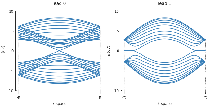
This is expected as lead 0 has armchair edges, while lead 1 has zigzag edges.
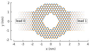
11.3. Fields in the leads
There is no need to specifically apply a field to a lead. Fields (and all modifier functions) are always applied globally to both the main system and all leads. For example, we can define a PN junction at \(x_0 = 0\) and pass it to the model:
def pn_junction(x0, v1, v2):
    @pb.onsite_energy_modifier
    def potential(energy, x):
        energy[x < x0] += v1
        energy[x >= x0] += v2
        return energy
    return potential

model = pb.Model(
    graphene.monolayer_4atom(),
    ring(0.8, 2),
    pn_junction(x0=0, v1=-1, v2=1)
)
model.attach_lead(direction=-1, contact=pb.line([-2, -1], [-2,  1]))
model.attach_lead(direction=+1, contact=pb.line([ 2, -1], [ 2,  1]))
model.plot()
We can view the potential applied to the main system using the Model.onsite_map property.
model.onsite_map.plot(cmap="coolwarm", site_radius=0.06)
pb.pltutils.colorbar(label="U (eV)")
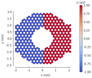
The appropriate potential is automatically applied to the leads depending on their position, left or right of the PN junction. We can quickly check this by plotting the band structure:
plt.figure(figsize=(6.7, 3))
plt.subplot(121)
model.leads[0].plot_bands()
plt.ylim(-10, 10)
plt.subplot(122)
model.leads[1].plot_bands()
plt.ylim(-10, 10)
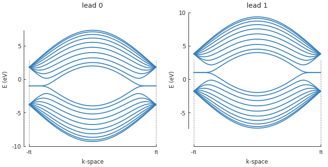
The leads are identical, except for a \(\pm1\) eV shift due to the PN junction, as expected.
11.4. Solving a scattering problem
At this time, pybinding doesn’t have a builtin solver for scattering problems. However, they can
be solved using Kwant. An arbitrary model can be constructed in
pybinding and then exported using the Model.tokwant() method. See the Kwant compatibility
page for details.
Alternatively, any user-defined solver and/or computation routine can be used. Pybinding generates
the model information in a standard CSR matrix format. The required Hamiltonian matrices are
Model.hamiltonian for the main scattering region and Lead.h0 and Lead.h1
for each of the leads found in Model.leads. For more information see the Model
and Lead API reference pages.